Instrumental variables II and regression discontinuity II
Materials for class on Monday, November 18, 2019
Contents
Slides
Download the slides from today’s class.

In-class R work
Open the RStudio.cloud project for today or download the project to your computer, unzip it, and run it locally:
ITT and CACE
Compliance
In class we talked about the difference between the average treatment effect (ATE), or the average effect of a program for an entire population, and conditional averages treatment effects (CATE), or the average effect of a program for some segment of the population. There are all sorts of CATEs: you can find the CATE for men vs. women, for people who are treated with the program (the average treatment on the treated, or ATT or TOT), for people who are not treated with the program (the average treatment on the untreated, or ATU), and so on.
One important type of CATE is the effect of a program on just those who comply with the program. We can call this the complier average treatment effect, but the acronym would be the same as conditional average treatment effect, so we’ll call it the conditional average causal effect (CACE).
Thinking about compliance is important. You might randomly assign people to receive treatment or a program, but people might not do what you tell them. Additionally, people might do the program if assigned to do it, but they would have done it anyway. We can split the population into four types of people:
- Compliers: People who follow whatever their assignment is (if assigned to treatment, they do the program; if assigned to control, they don’t)
- Always takers: People who will receive or seek out the program regardless of assignment (if assigned to treatment, they do the program; if assigned to control, they still do the program)
- Never takers: People who will not receive or seek out the program regardless of assignment (if assigned to treatment, they don’t do the program; if assigned to control, they also don’t do it)
- Defiers: People who will do the opposite of whatever their assignment is (if assigned to treatment, they don’t do the program; if assigned to control, they do the program)
To simplify things, evaluators and econometricians assume that defiers don’t exist based on the idea of monotonicity, which means that we can assume that the effect of being assigned to treatment only increases the likelihood of participating in the program (and doesn’t make it more likely).
The tricky part about trying to find who the compliers are in a sample is that we can’t know what people would have done in the absense of treatment. If we see that someone in the experiment was assigned to be in the treatment group and they then participated in the program, they could be a complier (since they did what they were assigned to do), or they could be an always taker (they did what they were assigned to do, but they would have done it anyway). Due to the fundamental problem of causal inference, we cannot know what each person would have done in a parallel world.
We can use data from a hypothetical program to see how these three types of compliers distort our outcomes.
library(tidyverse)
library(broom)
library(estimatr)

bed_nets <- read_csv("https://evalf19.classes.andrewheiss.com/data/bed_nets_observed.csv")
bed_nets_time_machine <- read_csv("https://evalf19.classes.andrewheiss.com/data/bed_nets_time_machine.csv")
This is what we would be able to see if we could read everyone’s minds. There are always takers who will use a bed net regardless of the program, and they’ll have higher health outcomes. However, those better outcomes are because of something endogenous—there’s something else that makes these people always pursue bed nets, and that’s likely related to health. We probably want to not consider them when looking for the program effect. There are never takers who won’t ever use a bed net, and they have worse health outcomes. Again, there’d endogeneity here—something is causing them to not use the bed nets, and it likely also causes their health level. We don’t want to look at them either.
The middle group—the compliers—are the people we want to focus on. Here we see that the program had an effect when compared to a control group.
ggplot(bed_nets_time_machine, aes(y = health, x = treatment)) +
  geom_point(aes(shape = bed_net, color = status), position = "jitter") +
  facet_wrap(~ status) +
  labs(color = "Type of person", shape = "Compliance",
       x = NULL, y = "Health status")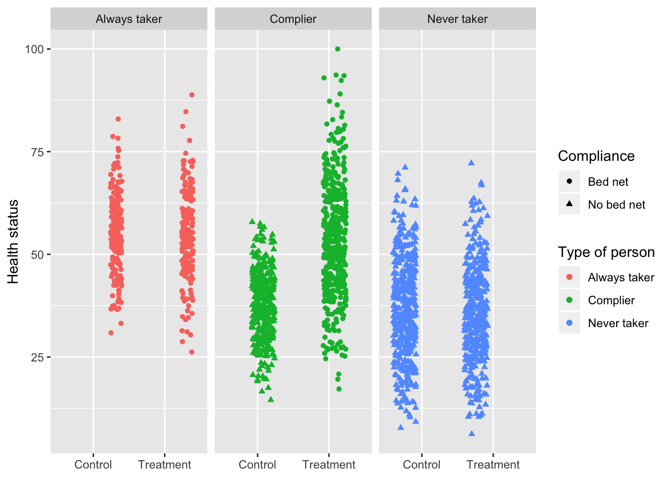
Finding compliers in actual data
This is what we actually see in the data, though. You can tell who some of the always takers are (those who used bed nets after being assigned to the control group) and who some of the never takers are (those who did not use a bed net after being assigned to the treatment group), but compliers are mixed up with the always and never takers. We have to somehow disentangle them!
ggplot(bed_nets_time_machine, aes(y = health, x = treatment)) +
  geom_point(aes(shape = bed_net, color = status), position = "jitter") +
  facet_wrap(~ bed_net) +
  labs(color = "Type of person", shape = "Compliance",
       x = NULL, y = "Health status")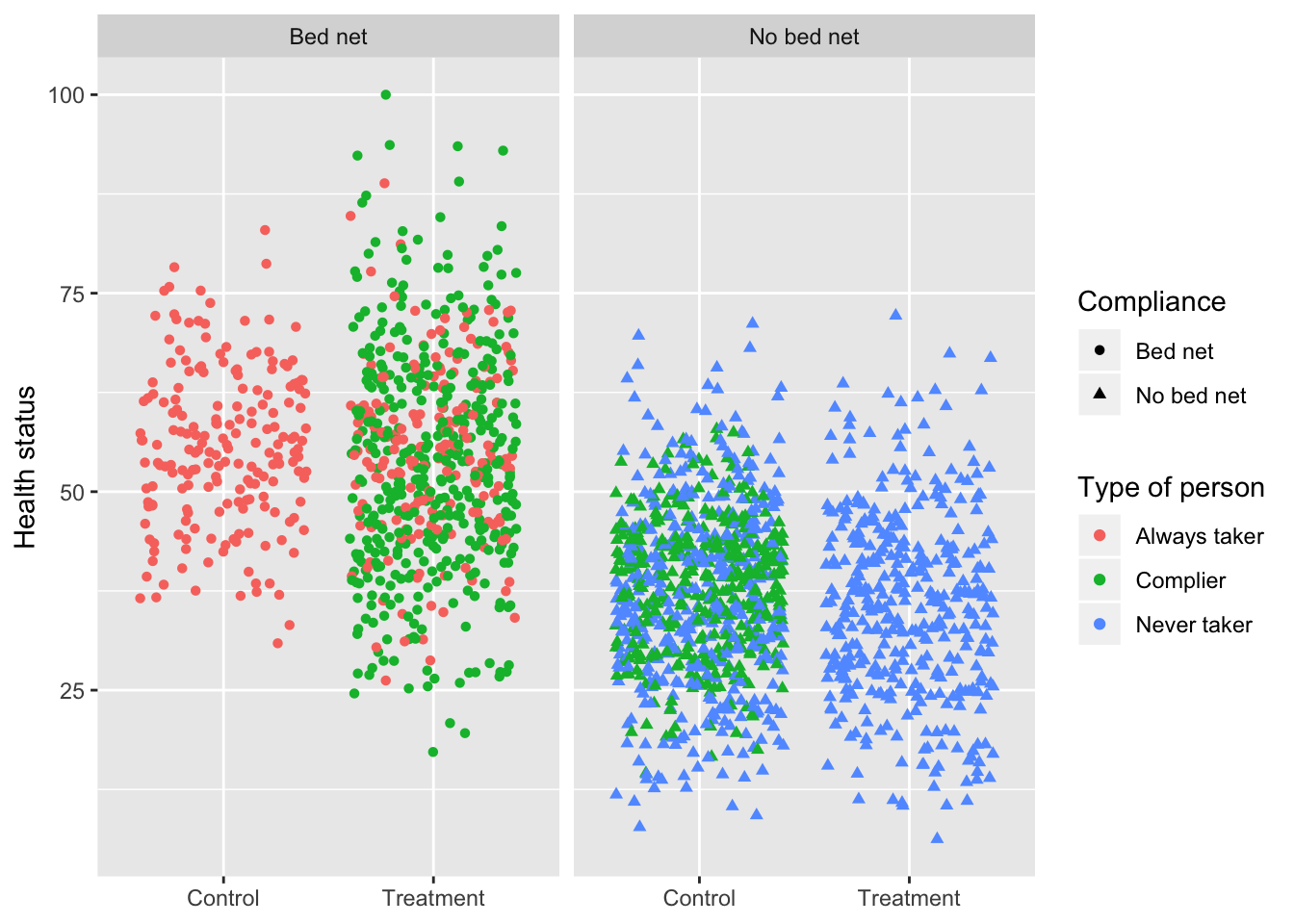
We can do this by assuming the proportion of compliers, never takers, and always takers are equally spread across treatment and control (which we can assume through the magic of randomization). If that’s the case, we can calculate the intent to treat (ITT) effect, which is the CATE of being assigned treatment (or the effect of being assigned treatment on health status, regardless of actual compliance).
The ITT is actually composed of three different causal effects: the complier average causal effect (CACE), the always taker average causal effect (ATACE), and the never taker average causal effect (NTACE). In the formula below, \(\pi\) stands for the proportion of people in each group. Formally, the ITT can be defined like this:
\[ \begin{aligned} \text{ITT} =& \pi_\text{compliers} \times (\text{T} - \text{C})_\text{compliers} + \\ &\pi_\text{always takers} \times (\text{T} - \text{C})_\text{always takers} + \\ &\pi_\text{never takers} \times (\text{T} - \text{C})_\text{never takers} \end{aligned} \]
We can simplify this to this acronymized version:
\[ \text{ITT} = \pi_\text{C} \text{CACE} + \pi_\text{A} \text{ATACE} + \pi_\text{N} \text{NTACE} \]
The number we care about the most here is the CACE, which is stuck in the middle of the equation. If we assume that assignment to treatment doesn’t make someone more likely to be an always taker or a never taker, we can set the ATACE and NTACE to zero, leaving us with just three variables to worry about: ITT, \(\pi_\text{c}\), and CACE:
\[ \begin{aligned} \text{ITT} =& \pi_\text{C} \text{CACE} + \pi_\text{A} 0 + \pi_\text{N} 0 \\ & \pi_\text{C} \text{CACE} \end{aligned} \]
We can use algebra to rearrange this formula so that we’re left with an equation that starts with CACE (since that’s the value we care about):
\[ \text{CACE} = \frac{\text{ITT}}{\pi_\text{C}} \]
If we can find the ITT and the proportion of compliers, we can find the complier average causal effect (CACE). The ITT is easy to find with a simple OLS model:
## # A tibble: 2 x 5
##   term               estimate std.error statistic  p.value
##   <chr>                 <dbl>     <dbl>     <dbl>    <dbl>
## 1 (Intercept)           40.9      0.444     92.1  0.
## 2 treatmentTreatment 5.99 0.630 9.51 5.36e-21The ITT here is ≈6—being assigned treatment increases average health status by 5.99 health points.
The proportion of compliers is a little trickier, but doable with some algebraic trickery. Recall from the graph above that the people who were in the treatment group and who complied are a combination of always takers and compliers. This means we can say:
\[ \begin{aligned} \pi_\text{A} + \pi_\text{C} =& \text{% in treatment and yes; or} \\ \pi_\text{C} =& \text{% in treatment and yes} - \pi_\text{A} \end{aligned} \]
We actually know \(\pi_\text{A}\)—remember in the graph above that the people who were in the control group and who used bed nets are guaranteed to be always takers (none of them are compliers or never takers). If we assume that the proportion of always takers is the same in both treatment and control, we can use that percent here, giving us this final equation for \(\pi_\text{C}\):
\[ \pi_\text{C} = \text{% in treatment and yes} - \text{% in control and yes} \]
So, if we can find the percent of people assigned to treatment who used bed nets, find the percent of people assigned to control and used bed nets, and subtract the two percentages, we’ll have the proportion of compliers, or \(\pi_\text{C}\). We can do that with the data we have (61% - 19.5% = 41.5% compliers):
## # A tibble: 4 x 4
## # Groups:   treatment [2]
##   treatment bed_net        n  prop
##   <chr>     <chr>      <int> <dbl>
## 1 Control   Bed net      196 0.195
## 2 Control   No bed net   808 0.805
## 3 Treatment Bed net      608 0.610
## 4 Treatment No bed net 388 0.390Finally, now that we know both the ITT and \(\pi_\text{C}\), we can find the CASE (or the LATE):
## [1] 14.42116It’s 14.4, which means that using bed nets increased health by 14 health points for compliers (which is a lot bigger than the 6 that we found before). We successfully filtered out the always takers and the never takers, and we have our complier-specific causal effect.
Finding the CASE/LATE with IV/2SLS
Doing that is super tedious though! What if there was an easier way to find the effect of the bed net program for just the compliers? We can do this with IV/2SLS regression by using assignment to treatment as an instrument.
Assignment to treatment works as an instrument because it’s (1) relevant, since being told to use bed nets is probably highly correlated with using bed nets, (2) exclusive, since the only way that being told to use bed nets can cause changes in health is through the actual use of the bed nets, and (3) exogenous, since being told to use bed nets probably isn’t related to other things that cause health.
Here’s a 2SLS regression with assignment to treatment as the instrument:
##                term  estimate std.error statistic      p.value  conf.low
## 1       (Intercept)  52.54401 0.8448045  62.19665 0.000000e+00  50.88722
## 2 bed_netNo bed net -14.42116 1.2538198 -11.50178 1.086989e-29 -16.88009
##   conf.high   df outcome
## 1  54.20080 1998  health
## 2 -11.96223 1998  health
The coefficient for bed_net is identical to the CACE that we found manually!It’s negative here because the base case is “Bed net” rather than “No bed net”.
Instrumental variables are helpful for isolated program effects to only compliers when you’re dealing with noncompliance.
Clearest and muddiest things
Go to this form and answer these three questions:
- What was the muddiest thing from class today? What are you still wondering about?
- What was the clearest thing from class today?
- What was the most exciting thing you learned?
I’ll compile the questions and send out answers after class.