Counterfactuals and DAGs II
Materials for class on Monday, September 30, 2019
Contents
Slides
Download the slides from today’s class.

In-class R work
Open the RStudio.cloud project for today or download the project to your computer, unzip it, and run it locally:
Making adjustments without using controls in regression
In 1986 Robert LaLonde published a report that studied the effect of a job training program on earnings in 1978. His study used an experiment to assign people to a training program or not, and he also collected data on people who voluntarily joined, which includes their earnings in 1975, prior to the training program. The wooldridge package in R contains this data.
library(tidyverse)
library(wooldridge)
library(ggdag)

# Clean the data
# The income variables here (re = real income) are measured in 1000s of dollars,
# so we adjust them into single dollars
randomly_assigned <- jtrain2 %>%
  mutate(re78 = re78 * 1000,
         re75 = re75 * 1000)

full_population <- jtrain3 %>%
  mutate(re78 = re78 * 1000,
         re75 = re75 * 1000)
We can check to see how much of an effect the job training program had on 1978 income by looking at the average income in both groups:
## # A tibble: 2 x 2
##   train avg_income
##   <int>      <dbl>
## 1     0      4555.
## 2     1      6349.
It looks like there’s an effect of almost $1,800:
## [1] 1794But what if we don’t have actual experimental data and are limited to just population data? Suppose we have a big dataset of people’s incomes, and some of them participated in a training program. Let’s check the group differences:
## # A tibble: 2 x 2
##   train avg_income
##   <int>      <dbl>
## 1     0     21554.
## 2     1      6349.
Here it looks like the training program had a substantial negative effect. The average income for people who didn’t receive the training is $21,500, while those who did get the training earn only $6,349.
There’s a confounder here though. The people who willingly participated in the training needed it for whatever reason—they may have been undereducated or undertrained or underexperienced, or something. If we compare this self-selected group to people who didn’t seek out training, we’re not comparing similar groups of people.
If we make a DAG, we can see that we need to adjust for “Needs training” since it’s a backdoor to income
# Possible DAG
training_dag <- dagify(wage ~ train + U + need_tr,
                       train ~ U + need_tr,
                       exposure = "train",
                       outcome = "wage",
                       labels = c("wage" = "Income", "train" = "Training program",
                                  "need_tr" = "Needs training", "U" = "Other things"))
ggdag(training_dag, use_labels = "label", text = FALSE, seed = 1234) +
  theme_dag()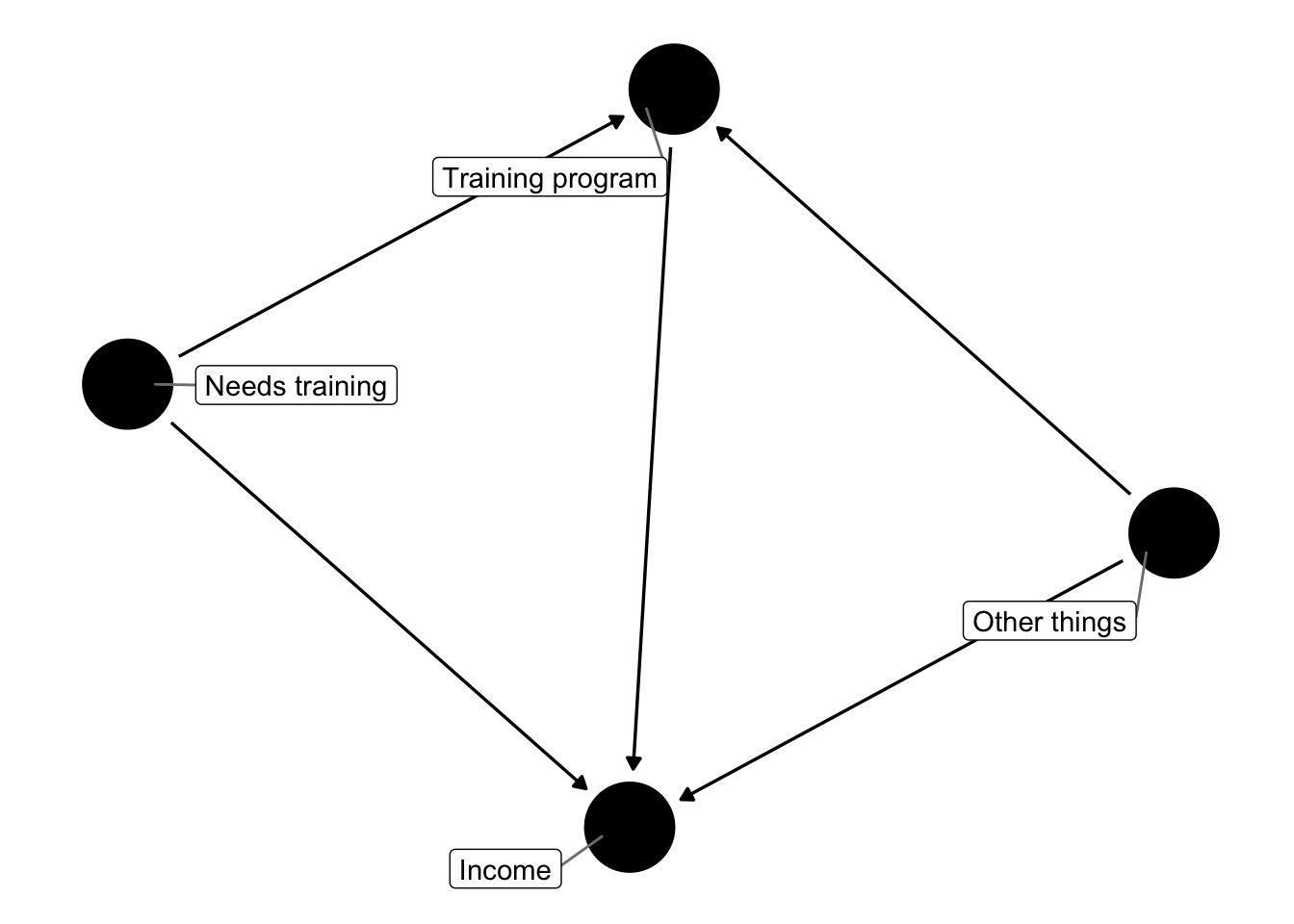
We don’t have a variable in our dataset named “Needs training,” but we can infer the need for training from pre-training income (like income in 1975 before the training program was offered).
Let’s look at the 1975 incomes of people in the experiment and the general population:
# The patchwork library lets you plot ggplots side-by-side by just using +. See
# https://github.com/thomasp85/patchwork for examples
#
# You can't install this like a normal package, since it's not in the central R
# package repository yet. You have to run these two lines to install it:
#
# install.packages("devtools")
# devtools::install_github("thomasp85/patchwork")

library(patchwork)

dist_random <- ggplot(randomly_assigned, aes(x = re75)) +
  geom_histogram(color = "white", binwidth = 1000) +
  labs(title = "Experiment", x = "1975 income", y = "Count")

dist_population <- ggplot(full_population, aes(x = re75)) +
  geom_histogram(color = "white", binwidth = 5000) +
  labs(title = "Full population", x = "1975 income", y = "Count")

dist_random + dist_population +
  plot_layout(ncol = 2)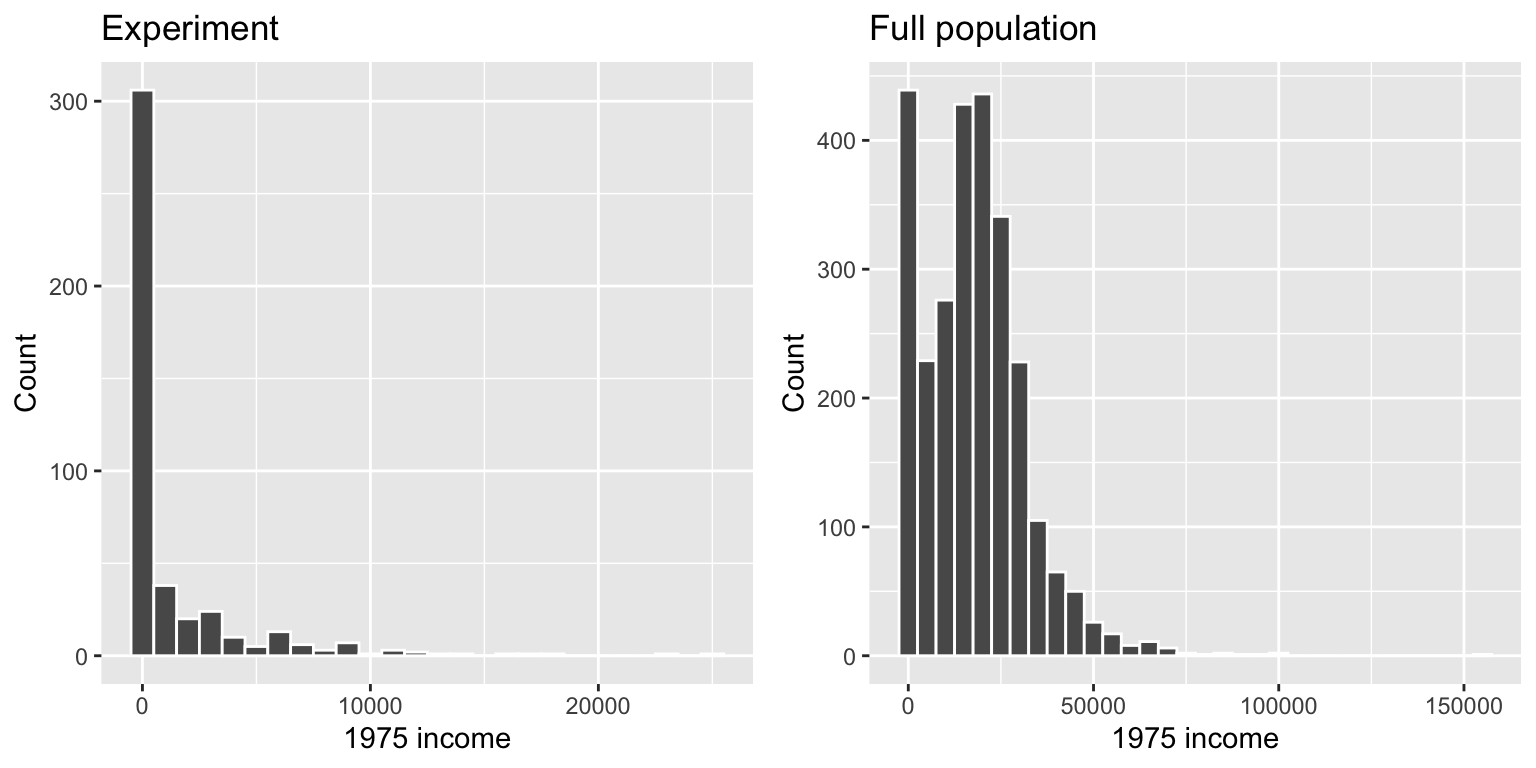
Those who participated in the experiment are much poorer on average than the total population, so we can infer that people in the regular world who have low incomes would need the job training.
We can adjust for “needs training” by limiting our sample of the full population to only those who have incomes below some threshold. There’s no official rule for what this threshold might be. In class, we looked at the different quartiles of income in the experiment group and found that the 75th percentile (3rd quartile) income was $1,221, which means that 75% of the people in the experiment had incomes of $1,221 or less.
##    Min. 1st Qu.  Median    Mean 3rd Qu.    Max.
##       0       0       0    1377    1221   25142
That sounds like a good threshold to start with, so let’s go with it. We can subset the full population using that threshold and then get the average income for people who did and did not receive training.
slice_of_population_needs_training <- full_population %>%
  filter(re75 < 1221)

slice_of_population_needs_training %>%
  group_by(train) %>%
  summarize(avg_income = mean(re78))
## # A tibble: 2 x 2
## train avg_income
## <int> <dbl>
## 1 0 5622.
## 2 1 5957.Now we have a more logical program effect. From this, after adjusting for whether people need the training (or holding need for training constant), we can see that the training program caused a small bump in income:
## [1] 335It’s a much smaller effect than what we found in the experiment, but we found it in the general population without running an actual experiment, which is kind of neat.
Is $1,221 a good threshold? I don’t know. We can play with it and see how much it affects the causal effect:
# Maybe 1,000 is a good number?
full_population %>%
  filter(re75 < 1000) %>%
  group_by(train) %>%
  summarize(avg_income = mean(re78))
## # A tibble: 2 x 2
## train avg_income
## <int> <dbl>
## 1 0 5652.
## 2 1 6037.# Or maybe 2,000?
full_population %>%
filter(re75 < 2000) %>%
group_by(train) %>%
summarize(avg_income = mean(re78))## # A tibble: 2 x 2
## train avg_income
## <int> <dbl>
## 1 0 5610.
## 2 1 6319.# Or maybe even 5,000?
full_population %>%
filter(re75 < 5000) %>%
group_by(train) %>%
summarize(avg_income = mean(re78))## # A tibble: 2 x 2
## train avg_income
## <int> <dbl>
## 1 0 6525.
## 2 1 6146.Clearest and muddiest things
Go to this form and answer these three questions:
- What was the muddiest thing from class today? What are you still wondering about?
- What was the clearest thing from class today?
- What was the most exciting thing you learned?
I’ll compile the questions and send out answers after class.