Threats to validity
Materials for class on Monday, October 7, 2019
Contents
Slides
Download the slides from today’s class.

Generating synthetic data
In class, I briefly demonstrated how to use the wakefield package to generate synthetic data for your final project.The package is named after Andrew Wakefield, a British researcher who used fake data to create a false link between the MMR vaccine and autism.
We’ll do more work with it later in the semester, but here’s a quick example of how to use it. You can find complete documentation at GitHub.
library(tidyverse)
library(wakefield)

# Make all the random draws consistent
set.seed(1234)

# The r_data_frame() function lets you generate random data. You just have to
# feed it the name of a function that generates variables. You can see all the
# possible variable-generating functions by running variables() in the R
# console:
variables()
## [1] "age" "animal" "answer"
## [4] "area" "car" "children"
## [7] "coin" "color" "date_stamp"
## [10] "death" "dice" "dna"
## [13] "dob" "dummy" "education"
## [16] "employment" "eye" "grade"
## [19] "grade_level" "group" "hair"
## [22] "height" "income" "internet_browser"
## [25] "iq" "language" "level"
## [28] "likert" "lorem_ipsum" "marital"
## [31] "military" "month" "name"
## [34] "normal" "political" "race"
## [37] "religion" "sat" "sentence"
## [40] "sex" "sex_inclusive" "smokes"
## [43] "speed" "state" "string"
## [46] "upper" "valid" "year"
## [49] "zip_code"# Here we generate a small data frame. Each of the functions that are listed in variables() has arguments. See age, for instance---we can specify a range of ages to draw from
small_data <- r_data_frame(
n = 30,
age(5:18), # Young kids
income(digits = 5), # Rich kids
zip_code,
race,
gender_inclusive
)
# Look at the first few rows
head(small_data)## # A tibble: 6 x 5
## Age Income Zip Race Gender
## <int> <dbl> <chr> <fct> <fct>
## 1 18 60519. 81105 White Trans*
## 2 8 203525. 17611 Black Male
## 3 8 94910. 17611 White Female
## 4 9 4744. 95858 White Female
## 5 12 76010. 56454 Hispanic Male
## 6 8 9534. 72651 White Trans*# You can make more complicated data too, like adding normally-distributed
# income, or assigning people to treatment and control groups
treatment <- r_data_frame(
n = 500,
race,
age(5:18),
income = rnorm(mean = 100000, sd = 15000) # Normal distribution centered at 100000
) %>%
mutate(treatment = "Yes")
control <- r_data_frame(
n = 500,
race,
age(5:18),
income = rnorm(mean = 50000, sd = 15000) # Normal distribution centered at 50000
) %>%
mutate(treatment = "No")
# We can combine these two datasets into one with bind_rows(), which essentially
# stacks the rows of one on top of the rows of the other:
big_data_set <- bind_rows(treatment, control)
# For fun, we can check the difference in income for people in the treatment and control groups
ggplot(big_data_set, aes(x = income, fill = treatment)) +
geom_density()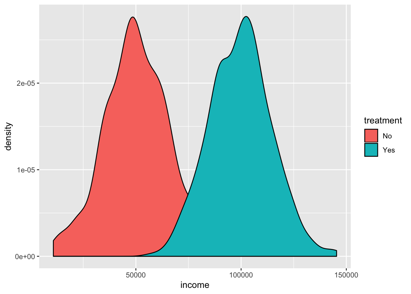
Whoa! Look at that! The imaginary program boosted incomes substantially! :)
In problem set 5 you worked with fake data about a hypothetical math camp. Here’s the code I used to generate that data. The only odd thing here is the rtruncnorm() function, which generates data from a truncated normal distribution. This makes it so you can put limits on numbers—if you want a random distribution of GPAs centered at 3.5, you don’t want to accidentally create GPAs of 4.3 or whatever. The a and b arguments let you set a minimum and a maximum number.
library(tidyverse)
library(wakefield)
library(rtruncnorm)

# Make all the random draws consistent
set.seed(1234)

# Treatment group with higher post-treatment GPA
treatment <- r_data_frame(n = 794,
                          id,
                          race,
                          age(x = 20:30),
                          gender_inclusive) %>%
  mutate(undergrad_gpa = round(rtruncnorm(n(), a = 1.0, b = 4.0,
                                          mean = 2.5, sd = .5), 2),
         math_camp = TRUE,
         gre_verbal = round(rtruncnorm(n(), a = 130, b = 170,
                                       mean = 145, sd = 15), 0),
         gre_quant = round(rtruncnorm(n(), a = 130, b = 170,
                                      mean = 110, sd = 15), 0),
         gre_total = gre_verbal + gre_quant,
         graduate_gpa = round(rtruncnorm(n(), a = 1.0, b = 4.0,
                                         mean = 3.3, sd = .5), 2))

# Control group with slightly higher post-treatment GPA
control <- r_data_frame(n = 787,
                        id,
                        race,
                        age(x = 20:30),
                        gender_inclusive) %>%
  mutate(undergrad_gpa = round(rtruncnorm(n(), a = 1.0, b = 4.0,
                                          mean = 2.5, sd = .5), 2),
         gre_verbal = round(rtruncnorm(n(), a = 130, b = 170,
                                       mean = 145, sd = 15), 0),
         gre_quant = round(rtruncnorm(n(), a = 130, b = 170,
                                      mean = 110, sd = 15), 0),
         math_camp = FALSE,
         gre_total = gre_verbal + gre_quant,
         graduate_gpa = round(rtruncnorm(n(), a = 1.0, b = 4.0,
                                         mean = 2.9, sd = .5), 2))

population <- r_data_frame(n = 1986,
                           id,
                           race,
                           age(x = 20:30),
                           gender_inclusive) %>%
  mutate(undergrad_gpa = round(rtruncnorm(n(), a = 1.0, b = 4.0,
                                          mean = 2.5, sd = 1.5), 2),
         gre_verbal = round(rtruncnorm(n(), a = 130, b = 170,
                                       mean = 145, sd = 15), 0),
         gre_quant = round(rtruncnorm(n(), a = 130, b = 170,
                                      mean = 160, sd = 30), 0),
         math_camp = FALSE,
         gre_total = gre_verbal + gre_quant,
         graduate_gpa = round(rtruncnorm(n(), a = 1.0, b = 4.0,
                                         mean = 3.6, sd = 1), 2))

# Combine them all
experiment <- bind_rows(treatment, control) %>%
  sample_frac(1)  # Shuffle the dataset for kicks and giggles

everyone <- bind_rows(experiment, population) %>%
  sample_frac(1)

# Save these as CSV files
write_csv(experiment, "math_camp_experiment.csv")
write_csv(everyone, "math_camp_everyone.csv")
Clearest and muddiest things
Go to this form and answer these three questions:
- What was the muddiest thing from class today? What are you still wondering about?
- What was the clearest thing from class today?
- What was the most exciting thing you learned?
I’ll compile the questions and send out answers after class.